Detecting Controllers’ Actions in Past Mode S Data by Autoencoder-Based Anomaly Detection
Xavier Olive, Jeremy Grignard, Thomas Dubot and Julie Saint-Lot
The dataset
The basic dataset consists of one year of trajectories between Paris Orly and Toulouse Blagnac airports. A learning box is arbitrarily defined so as to include about 20 minutes of flight before entering the TMA.
from traffic.core import Traffic
from shapely.geometry import box

# Data: one year of traffic between LFPO and LFBO
t = Traffic.from_file("data/2017_lfpo_lfbo.pkl")

# The learning box has been set manually on the data
learning_box = box(
    0.9488888502120971,
    44.287776947021484,
    2.748888850212097,
    45.537776947021484
)
The data has been downloaded from the OpenSky Network Impala database. The following recalls all the callsigns selected for this route.
# Pretty-print all the callsigns analysed

cs = sorted(t.callsigns)
for i in range(4):
    print(" ".join(cs[7*i:7*(i+1)]))
AF128UU AFR21ME AFR22MT AFR22SR AFR26SA AFR27GH AFR38DV
AFR43LC AFR47FW AFR49DL AFR51ZU AFR52BW AFR53TQ AFR57XL
AFR59UB AFR611H AFR613R AFR61JJ AFR61UJ AFR65WA AFR77PQ
AFR88DM EZY24EH EZY289N EZY353H EZY4019 EZY4029 EZY98KP
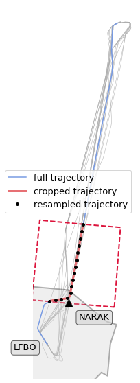
Data preparation
The following plot explains how each trajectory is prepared. The basic idea is to clip the trajectory to the learning box, then to resample each trajectory to a fixed number of samples (15 on the figure, 150 for the machine learning method).
import matplotlib.pyplot as plt

from traffic.data import airports, navaids, nm_airspaces
from cartes.crs import EuroPP, PlateCarree

with plt.style.context("traffic"):

    fig, ax = plt.subplots(subplot_kw=dict(projection=EuroPP()))

    ax.add_geometries(
        [learning_box],
        crs=PlateCarree(),
        facecolor="None",
        edgecolor="crimson",
        linewidth=2,
        linestyle="dashed",
    )

    # TMA of Toulouse Airport
    nm_airspaces["LFBOTMA"].plot(
        ax, edgecolor="black", facecolor="#cccccc", alpha=.3, linewidth=2
    )

    # Beacon marking the beginning of the STAR procedure
    navaids["NARAK"].plot(
        ax,
        zorder=2,
        marker="^",
        shift=dict(units="dots", x=15, y=-15),
        text_kw={
            "s": "NARAK",
            "verticalalignment": "top",
            "bbox": dict(facecolor="lightgray", alpha=0.6, boxstyle="round"),
        },
    )

    airports["LFBO"].point.plot(
        ax,
        shift=dict(units="dots", x=-15),
        alpha=0,
        text_kw=dict(
            s="LFBO",
            verticalalignment="top",
            horizontalalignment="right",
            bbox=dict(facecolor="lightgray", alpha=0.6, boxstyle="round"),
        ),
    )

    # Few trajectories from the data set
    t.plot(ax, color="#aaaaaa", zorder=-2, linewidth=.6, nb_flights=20)

    # Details of the data preparation
    t["EZY24EH_2831"].plot(ax, linewidth=1.5, label="full trajectory")
    t["EZY24EH_2831"].clip(learning_box).plot(
        ax, linewidth=3, label="cropped trajectory"
    )
    t["EZY24EH_2831"].clip(learning_box).resample(15).plot(
        ax,
        linewidth=0,
        marker=".",
        color="black",
        label="resampled trajectory",
    )

    ax.legend()
    ax.spines['geo'].set_visible(False)
    ax.background_patch.set_visible(False)
The following applies the preprocessing to each trajectory in the dataset.
t_clip = Traffic.from_flights(
    flight
    # Median filters on all trajectories
    .filter()
    # Clipping to the learning box
    .clip(learning_box)
    # Resample to 150 samples per flight
    .resample(150)
    for flight in t
)
# Backup to one file
t_clip.to_pickle("data/2017_lfpo_lfbo_prepared.pkl")
t_clip = Traffic.from_file("data/2017_lfpo_lfbo_prepared.pkl")
t_clip
| count | |
|---|---|
| flight_id | |
| AF128UU_073 | 150 |
| AFR77PQ_1064 | 150 |
| AFR77PQ_1012 | 150 |
| AFR77PQ_1013 | 150 |
| AFR77PQ_1014 | 150 |
| AFR77PQ_1015 | 150 |
| AFR77PQ_1016 | 150 |
| AFR77PQ_1058 | 150 |
| AFR77PQ_1059 | 150 |
| AFR77PQ_1060 | 150 |
Machine-Learning
The anomaly detection method is based on a shallow autoencoder (PyTorch implementation). For the sake of this example, we focus on the track angle signal. At the end of the training period, we look at the distribution of the reconstruction errors.
import numpy as np

from sklearn.preprocessing import minmax_scale
from torch import from_numpy, nn, optim
from torch.autograd import Variable
from tqdm.autonotebook import tqdm

# -- Autoencoder architecture --

class Autoencoder(nn.Module):
    """Basic shallow autoencoder."""
    def __init__(self):
        super().__init__()
        self.encoder = nn.Sequential(
            nn.Linear(150, 64),
            # Activation function
            nn.Sigmoid()
        )
        self.decoder = nn.Sequential(
            nn.Linear(64, 150),
            # Activation function
            nn.Sigmoid()
        )

    def forward(self, x, **kwargs):
        x = self.encoder(x)
        x = self.decoder(x)
        return x


def anomalies(t: Traffic):

    flight_ids = list(f.flight_id for f in t)

    # For this example, we only work on the track angle signal
    X = minmax_scale(np.vstack(f.data.track for f in t))

    model = Autoencoder().cuda()
    criterion = nn.MSELoss()
    optimizer = optim.Adam(model.parameters(), lr=1e-3, weight_decay=1e-5)

    # Basic training process (GPU)
    loss_evolution = []
    for epoch in tqdm(range(2000)):

        v = Variable(from_numpy(X.astype(np.float32))).cuda()
        output = model(v)
        loss = criterion(output, v)
        loss_evolution.append(loss.data.item())

        optimizer.zero_grad()
        loss.backward()
        optimizer.step()

    output = model(v)
    # Compute the reconstruction error for each flight
    errors = dict(
        (id_, err)
        for id_, err in zip(
            flight_ids,
            (nn.MSELoss(reduction="none")(output, v).sum(1))
            .sqrt()
            .cpu()
            .detach()
            .numpy(),
        )
    )
    return errors, loss_evolution
Now we apply the anomaly detection on the preprocessed data and analyse the distribution as explained in the paper.
errors, loss_evolution = anomalies(t_clip)

with plt.style.context("traffic"):
    fig, (ax1, ax2, ax3) = plt.subplots(3, 1, figsize=(10, 21))
    ax1.plot(loss_evolution)
    ax2.hist(errors.values(), bins=20)
    h = ax3.hist(errors.values(), bins=20)
    ax3.set_yscale("log")

    for i, id_ in enumerate(
        [
            "EZY24EH_3324",
            "AFR47FW_2174",
            "AFR61UJ_1321",
            "AFR27GH_348",
            "AFR51ZU_027",
        ]
    ):
        ax3.annotate(
            f"{t[id_].callsign}, {t[id_].stop:%b %d}",
            xy=(errors[id_], h[0][sum(h[1] - errors[id_] < 0) - 1]),
            xytext=(errors[id_], 2 ** (i + 3)),
            fontsize=16,
            horizontalalignment="left",
            arrowprops=dict(
                arrowstyle="->", connectionstyle="arc,angleA=180,armA=70,rad=10"
            ),
        )

    ax1.set_xlabel("Number of epochs", labelpad=10)
    ax1.set_ylabel("Loss evolution")
    ax2.set_ylabel("Number of samples")
    ax3.set_ylabel("Number of samples")
    ax3.set_xlabel("Reconstruction error", labelpad=10)
