Getting started
The motivation for this page/notebook is to take the reader through all basic functionalities of the traffic library. In particular, we will cover:
a basic introduction about
FlightandTrafficstructures;how to produce visualisations of trajectory data;
a use case to display trajectories around Paris area;
an introduction to declarative trajectory processing through lazy iteration
Tip
This page is also available as a notebook which can be
downloaded and executed locally;
or loaded and executed in Google Colab.
Basic introduction
The traffic library provides natural methods and attributes that can be applied on trajectories and collection of trajectories, all represented as pandas DataFrames.
Flight objects
Flightis the core class offering representations, methods and attributes to single trajectories. Trajectories can either:
be imported from the sample trajectory set;
be downloaded from OpenSky Impala shell;
be loaded from a tabular file (csv, json, parquet, etc.);
be decoded from raw ADS-B signals.
The Belevingsvlucht from the sample trajectory set is present throughout the documentation:
from traffic.data.samples import belevingsvluchtMany representations are available:
in a Python interpreter:
print(belevingsvlucht)Flight(icao24='484506', callsign='TRA051')with rich simple or advanced representations:
from rich.pretty import pprint pprint(belevingsvlucht)Flight(icao24='484506', callsign='TRA051')# the console is not necessary if you ran pretty.install() from rich.console import Console console = Console() console.print(belevingsvlucht)Flight - callsign: TRA051 - aircraft: 484506 · 🇳🇱 PH-HZO (B738) - start: 2018-05-30 15:21:38Z - stop: 2018-05-30 20:22:56Z - duration: 0 days 05:01:18 - sampling rate: 1 second(s) - features: o altitude, int64 o groundspeed, int64 o latitude, double o longitude, double o timestamp, timestamp o track, int64 o vertical_rate, int64
- in a Jupyter notebook:
belevingsvluchtFlight
- callsign: TRA051
- aircraft:
484506· 🇳🇱 PH-HZO (B738)- start: 2018-05-30 15:21:38+00:00
- stop: 2018-05-30 20:22:56+00:00
- duration: 0 days 05:01:18
- sampling rate: 1 second(s)
Information about each
Flightis available through attributes or properties:dict(belevingsvlucht){'callsign': 'TRA051', 'icao24': '484506', 'aircraft': Tail(icao24='484506', registration='PH-HZO', typecode='B738', flag='🇳🇱'), 'start': Timestamp('2018-05-30 15:21:38+0000', tz='UTC'), 'stop': Timestamp('2018-05-30 20:22:56+0000', tz='UTC'), 'duration': Timedelta('0 days 05:01:18')}Methods are provided to select relevant parts of the flight, e.g. based on timestamps. The
startandstopproperties refer to the timestamps of the first and last recorded samples. Note that all timestamps are by default set to universal time (UTC) as it is common practice in aviation.(belevingsvlucht.start, belevingsvlucht.stop)(Timestamp('2018-05-30 15:21:38+0000', tz='UTC'), Timestamp('2018-05-30 20:22:56+0000', tz='UTC'))belevingsvlucht.first(minutes=30)Flight
- callsign: TRA051
- aircraft:
484506· 🇳🇱 PH-HZO (B738)- start: 2018-05-30 15:21:38+00:00
- stop: 2018-05-30 15:51:37+00:00
- duration: 0 days 00:29:59
- sampling rate: 1 second(s)
Warning
Note the difference between the “strict” comparison (\(>\)) vs. “or equal” comparison (\(\geq\))
belevingsvlucht.after("2018-05-30 19:00", strict=False)Flight
- callsign: TRA051
- aircraft:
484506· 🇳🇱 PH-HZO (B738)- start: 2018-05-30 19:00:00+00:00
- stop: 2018-05-30 20:22:56+00:00
- duration: 0 days 01:22:56
- sampling rate: 1 second(s)
Note
Each
Flightis wrapped around apandas.DataFrame: when no method is available for your particular need, you can always access the underlying dataframe.belevingsvlucht.between("2018-05-30 19:00", "2018-05-30 20:00").data
timestamp icao24 latitude longitude groundspeed track vertical_rate callsign altitude 11750 2018-05-30 19:00:01+00:00 484506 52.839973 5.793947 290 52 -1664 TRA051 8233 11751 2018-05-30 19:00:02+00:00 484506 52.840747 5.79568 290 52 -1664 TRA051 8200 11752 2018-05-30 19:00:03+00:00 484506 52.841812 5.797501 290 52 -1664 TRA051 8200 11753 2018-05-30 19:00:04+00:00 484506 52.842609 5.799133 290 52 -1599 TRA051 8149 11754 2018-05-30 19:00:05+00:00 484506 52.843277 5.80101 289 52 -1599 TRA051 8125 ... ... ... ... ... ... ... ... ... ... 14750 2018-05-30 19:59:54+00:00 484506 52.84964 5.357513 277 280 0 TRA051 6000 14751 2018-05-30 19:59:56+00:00 484506 52.850104 5.351205 277 277 640 TRA051 6025 14752 2018-05-30 19:59:57+00:00 484506 52.850281 5.349197 277 277 640 TRA051 6050 14753 2018-05-30 19:59:58+00:00 484506 52.85043 5.347046 277 277 1088 TRA051 6050 14754 2018-05-30 19:59:59+00:00 484506 52.850601 5.344849 278 277 1216 TRA051 6075 3005 rows × 9 columns
Traffic objects
Trafficis the core class to represent collections of trajectories. In practice, all trajectories are flattened in the samepandas.DataFrame.from traffic.data.samples import quickstartThe basic representation of a
Trafficobject is a summary view of the data: the structure tries to infer how to separate trajectories in the data structure based on customizable heuristics, and returns a number of sample points for each trajectory.quickstartTraffic
with 236 identifiers
count icao24 callsign 39d300 TVF91KQ 3893 39b002 FHMAC 3360 3aabfc FMY8055 2669 39c82b PEA501 2247 4241bb VPCAL 2168 02a195 TAR722 2166 398495 CCM774V 2134 4bc844 PGT90Y 2124 39ceb4 TVF19YP 2076 4d02be JFA12P 2057 Trafficobjects offer the ability to index and iterate on all flights contained in the structure.
a customizable flight identifier (
flight_id); ora combination of
timestampandicao24(aircraft identifier);Indexation will be made on:
icao24,callsign(orflight_idif available):quickstart["TAR722"] # return type: Flight, based on callsign quickstart["39b002"] # return type: Flight, based on icao24Flight
- callsign: FHMAC
- aircraft:
39b002· 🇫🇷 F-HMAC (EC20)- start: 2021-10-07 13:21:56+00:00
- stop: 2021-10-07 14:17:57+00:00
- duration: 0 days 00:56:01
- sampling rate: 1 second(s)
an integer or a slice, to take flights in order in the collection:
quickstart[0] # return type: Flight, the first trajectory in the collection quickstart[:10] # return type: Traffic, the 10 first trajectories in the collectionTraffic
with 10 identifiers
count icao24 callsign 02a195 TAR722 2166 0a0046 DAH1011 1323 0101de MSR799 1290 34150e IBE34AK 1152 06a2b1 QTR9UU 1144 0a0047 DAH1000 1111 300789 IWALK 1024 06a1e7 QTR23JR 874 06a133 QQE940 803 0a0047 DAH1001 798 a subset of trajectories can also be selected:
if a list is passed an index:
quickstart[['AFR83HQ', 'AFR83PX', 'AFR84UW', 'AFR91QD']]Traffic
with 4 identifiers
count icao24 callsign 394c04 AFR83PX 1274 3946e2 AFR84UW 1112 3946e0 AFR91QD 1078 3950d0 AFR83HQ 650 with a pandas-like
query():quickstart.query('callsign.str.startswith("AFR")')Traffic
with 84 identifiers
count icao24 callsign 393324 AFR69CR 1992 393320 AFR85FF 1975 398564 AFR9455 1666 3985a4 AFR19BH 1636 3944f1 AFR15AH 1546 3944f0 AFR51LU 1525 393321 AFR18KJ 1486 3944ed AFR71ZP 1463 3950cd AFR26TR 1396 394c13 AFR1753 1346 There are several ways to assign a flight identifier. The most simple one that you will use in 99% of situations involves the
flight_id()method.quickstart.assign_id().eval()Traffic
with 238 identifiers
count flight_id TVF91KQ_137 3893 FHMAC_116 3360 VPCAL_156 2168 TAR722_001 2166 CCM774V_087 2134 PGT90Y_196 2124 TVF19YP_134 2076 JFA12P_207 2057 AFR69CR_025 1992 AFR85FF_023 1975
Data visualization
The traffic library offers facilities to leverage the power of common visualization renderers including Matplotlib and Altair.
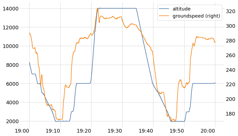
with Matplotlib, the
trafficstyle context (optional) offers a convenient initial stylesheet:import matplotlib.pyplot as plt from matplotlib.dates import DateFormatter with plt.style.context("traffic"): fig, ax = plt.subplots(figsize=(10, 7)) ( belevingsvlucht .between("2018-05-30 19:00", "2018-05-30 20:00") .plot_time( ax=ax, y=["altitude", "groundspeed"], secondary_y=["groundspeed"] ) ) ax.set_xlabel("") ax.tick_params(axis='x', labelrotation=0) ax.xaxis.set_major_formatter(DateFormatter("%H:%M"))
- The
chart()method triggers an initial representation with Altair which can be further refined.For example, with the following subset of trajectories:subset = quickstart[["TVF22LK", "EJU53MF", "TVF51HP", "TVF78YY", "VLG8030"]]
subset[0].chart()
Even a simple visualization without a physical features plotted on the y-channel can be meaningful. The following proposition helps visualizing when aircraft are airborne:
import altair as alt # necessary line if you see an error about a maximum number of rows alt.data_transformers.disable_max_rows() alt.layer( *( flight.chart().encode( alt.Y("callsign", sort="x", title=None), alt.Color("callsign", legend=None), ) for flight in subset ) ).configure_line(strokeWidth=4)
The y-channel is however most often used to plot physical quantities such as altitude, ground speed, or more.
alt.layer( *( flight.chart().encode( alt.Y("altitude"), alt.Color("callsign"), ) for flight in subset ) )
Simple plots are beautiful by default, but it is still possible to further refine them. For more advanced tricks with Altair, refer to their online documentation.
chart = ( alt.layer( *( flight.chart().encode( alt.X( "utcdayhoursminutesseconds(timestamp)", axis=alt.Axis(format="%H:%M"), title=None, ), alt.Y("altitude", title=None, scale=alt.Scale(domain=(0, 18000))), alt.Color("callsign"), ) for flight in subset ) ) .properties(title="altitude (in ft)") # "trick" to display the y-axis title horizontally .configure_legend(orient="bottom") .configure_title(anchor="start", font="Lato", fontSize=16) ) chart
Making maps
Maps are also available with Matplotlib, Altair, and thanks to ipyleaflet widgets.
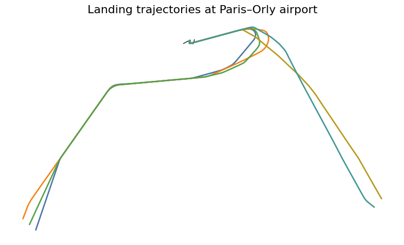
with Matplotlib, you need to specify a projection for your axis system. They are provided by cartes on top of Cartopy. Here, the Lambert93 projection is picked as it is a standard projection in France.
All traffic objects which may be represented on a map are equipped with a
plot()method.from cartes.crs import Lambert93 from traffic.data import airports with plt.style.context("traffic"): fig, ax = plt.subplots(subplot_kw=dict(projection=Lambert93())) airports["LFPO"].plot(ax, footprint=False, runways=dict(linewidth=1)) for flight in subset: flight.plot(ax, linewidth=2) ax.set_title("Landing trajectories at Paris–Orly airport")
with Altair, the initial method is
geoencode()from traffic.data import airports chart = ( alt.layer( *(flight.geoencode().encode(alt.Color("callsign:N")) for flight in subset) ) .properties(title="Landing trajectories at Paris–Orly airport") .configure_legend(orient="bottom") .configure_view(stroke=None) .configure_title(anchor="start", font="Lato", fontSize=16) ) chart
for quick interactive representations with few elements, the Leaflet widget is a good option:
subset.map_leaflet(zoom=8)
Low-altitude trajectory patterns in Paris metropolitan area
The quickstart dataset contains a collection of low altitude trajectories.
In this section, we aim to display trajectory patterns of aircraft landing or
taking off from any of Paris area airport.
It is often a good practice to just plot the data as is before we get an idea of how to proceed.
with plt.style.context("traffic"):
fig, ax = plt.subplots(subplot_kw=dict(projection=Lambert93()))
quickstart.plot(ax, alpha=.7)
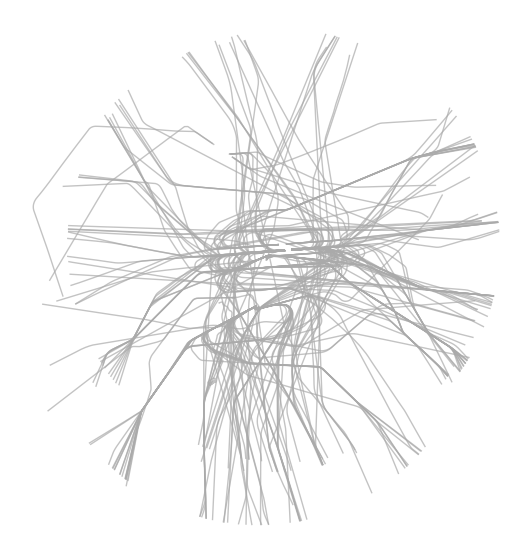
We see here several flows converging mostly in the two major airports in Paris
(i.e., Orly LFPO and Charles-de-Gaulle LFPG). However, more airports are
also visible, e.g. Beauvais airport to the North.
We can try to put a different colour to landing trajectories and take-off trajectories to make this plot more meaningful. A first trick could be to pick a colour based on the vertical rate average value.
import pandas as pd
with plt.style.context("traffic"):
fig, ax = plt.subplots(subplot_kw=dict(projection=Lambert93()))
for flight in quickstart:
if pd.isna(flight.vertical_rate_mean):
continue
if flight.vertical_rate_mean < -500:
flight.plot(ax, color="#4c78a8", alpha=0.5) # blue
elif flight.vertical_rate_mean > 1000:
flight.plot(ax, color="#f58518", alpha=0.5) # orange
else:
flight.plot(ax, color="#54a24b", alpha=0.5) # green
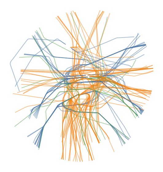
This approach is not perfect (there are quite some green trajectories) but gives
a good first idea of how traffic organizes itself. Let’s try to focus on the
traffic to and from one airport, e.g. LFPO, in order to refine the
methodology.
A first approach to select those trajectories would be to pick the first/last
point of the Flight and check whether it falls within the
geographical scope of the airport. In the following snippet, we do things a bit
differently: we check whether the first/last 5 minutes of the trajectory
intersects the shape of the airport.
from traffic.data import airports
with plt.style.context("traffic"):
fig, ax = plt.subplots(subplot_kw=dict(projection=Lambert93()))
for flight in quickstart:
if pd.isna(flight.vertical_rate_mean):
continue
if flight.vertical_rate_mean < -500:
if flight.last("5 min").intersects(airports["LFPO"]):
flight.plot(ax, color="#4c78a8", alpha=0.5)
elif flight.vertical_rate_mean > 1000:
if flight.first("5 min").intersects(airports["LFPO"]):
flight.plot(ax, color="#f58518", alpha=0.5)
What is now becoming confusing is that there seems to have been a change in runway configuration during the time interval covered by the dataset. It would now probably become more comfortable if we could identify the runway used by aircraft for take off or landing.
traffic provides landing() for landing and
takeoff() for take-off. Both methods
return a FlightIterator(), so if we consider that all
trajectories have only one landing attempt on that day, we need to apply
next() to get the first trajectory segment
matching, and extract relevant information (the runway information):
import pandas as pd
from tqdm.rich import tqdm
information = list()
for flight in tqdm(quickstart):
if landing := flight.landing("LFPO").next():
information.append(
{
"callsign": flight.callsign,
"icao24": flight.icao24,
"airport": "LFPO",
"stop": landing.stop,
"ILS": landing.ILS_max,
}
)
elif landing := flight.landing("LFPG").next():
information.append(
{
"callsign": flight.callsign,
"icao24": flight.icao24,
"airport": "LFPG",
"stop": landing.stop,
"ILS": landing.ILS_max,
}
)
elif landing := flight.landing("LFPB").next():
information.append(
{
"callsign": flight.callsign,
"icao24": flight.icao24,
"airport": "LFPB",
"stop": landing.stop,
"ILS": landing.ILS_max,
}
)
stats = pd.DataFrame.from_records(information)
stats
| callsign | icao24 | airport | stop | ILS | |
|---|---|---|---|---|---|
| 0 | MSR799 | 0101de | LFPG | 2021-10-07 12:34:22+00:00 | 26L |
| 1 | TAR722 | 02a195 | LFPO | 2021-10-07 14:25:04+00:00 | 06 |
| 2 | QTR9UU | 06a2b1 | LFPG | 2021-10-07 12:42:49+00:00 | 26L |
| 3 | DAH1000 | 0a0047 | LFPG | 2021-10-07 12:27:55+00:00 | 26L |
| 4 | AEA1297 | 344487 | LFPO | 2021-10-07 14:33:14+00:00 | 06 |
| ... | ... | ... | ... | ... | ... |
| 86 | SVA127 | 7103d7 | LFPG | 2021-10-07 14:54:46+00:00 | 08R |
| 87 | JAL45 | 86e430 | LFPG | 2021-10-07 14:29:35+00:00 | 08R |
| 88 | FDX5046 | a06310 | LFPG | 2021-10-07 14:59:59+00:00 | 09R |
| 89 | AMX003 | a560f3 | LFPG | 2021-10-07 14:27:00+00:00 | 08R |
| 90 | FDX5093 | ab8b7f | LFPG | 2021-10-07 14:42:25+00:00 | 09R |
91 rows × 5 columns
chart = (
alt.Chart(stats)
.encode(
alt.X("utcdayhoursminutesseconds(stop)", axis=alt.Axis(format="%H:%M"), title=None),
alt.Y("ILS", title=None),
alt.Color("ILS", legend=None),
alt.Row("airport", title=None),
)
.mark_square(size=80)
.resolve_scale(y="independent")
.configure_header(
labelOrient="top",
labelAnchor="start",
labelFont="Lato",
labelFontWeight="bold",
labelFontSize=16,
)
.configure_axis(labelFontSize=13)
.properties(width=600)
)
chart
It appears here that there has been a coordinated runway configuration change around 13:20Z in all Paris airports. This suggests we should plot how traffic organizes in both configurations.
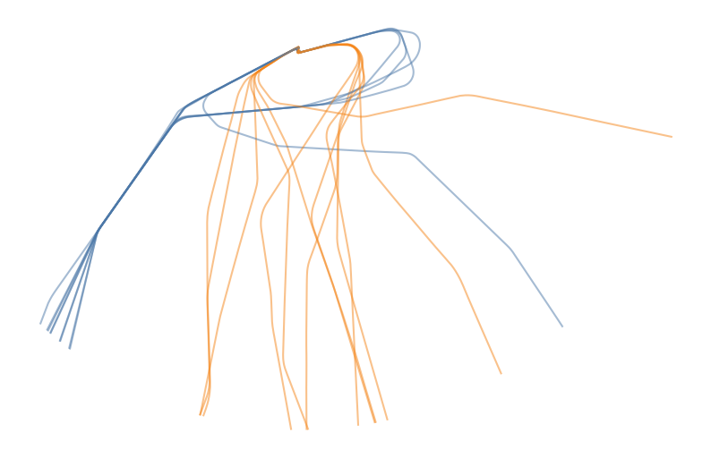
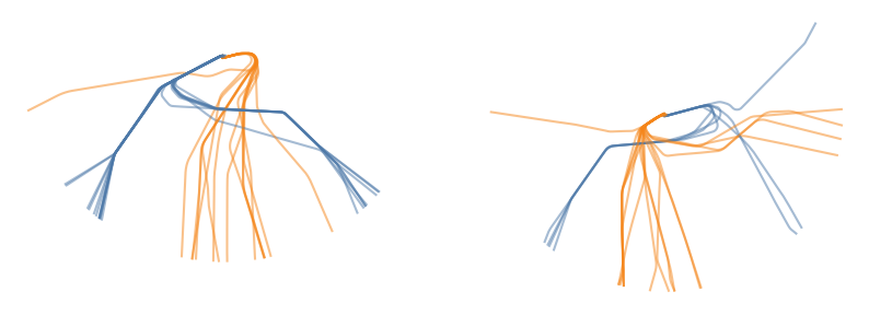
with plt.style.context("traffic"):
fig, ax = plt.subplots(1, 2, subplot_kw=dict(projection=Lambert93()))
for flight in quickstart:
if segment := flight.landing("LFPO").next():
index = int(flight.stop <= pd.Timestamp("2021-10-07 13:30Z"))
flight.plot(ax[index], color="#4c78a8", alpha=0.5)
elif segment := flight.takeoff("LFPO").next():
index = int(segment.start <= pd.Timestamp("2021-10-07 13:20Z"))
flight.plot(ax[index], color="#f58518", alpha=0.5)
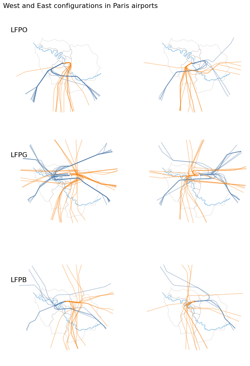
So it is now time to do a preliminary visualization with a basic background, including administrative boundaries of Greater Paris Area and the Seine river as an additional landmark:
from cartes.atlas import france
from cartes.crs import Lambert93, PlateCarree
from cartes.osm import Nominatim
# background elements
paris_area = france.data.query("ID_1 == 1000")
seine_river = (
Nominatim.search("Seine river, France")
.shape.intersection(
paris_area.union_all().buffer(0.1)
)
)
with plt.style.context("traffic"):
fig, ax = plt.subplots(
3, 2, figsize=(10, 15), subplot_kw=dict(projection=Lambert93())
)
airport_codes = ["LFPO", "LFPG", "LFPB"]
for flight in quickstart:
phases = flight.phases()
if phases.query('phase == "DESCENT"'):
# Determine on which ax to plot based on detected airport
for airport_index, airport in enumerate(airport_codes):
if segment := flight.landing(airport).next():
# Determine on which column to plot based on time
time_index = int(segment.stop <= pd.Timestamp("2021-10-07 13:20Z"))
flight.plot(
ax[airport_index, time_index], color="#4c78a8", alpha=0.4
)
break
elif phases.query('phase == "CLIMB"'):
# Determine on which ax to plot based on detected airport
for airport_index, airport in enumerate(airport_codes):
if segment := flight.takeoff(airport).next():
# Determine on which column to plot based on time
time_index = int(segment.start <= pd.Timestamp("2021-10-07 13:20Z"))
flight.plot(
ax[airport_index, time_index], color="#f58518", alpha=0.4
)
break
# Annotate each map with airport information
for i, airport in enumerate(airport_codes):
ax[i, 0].set_title(f"{airport}", loc="left", y=0.8)
for ax_ in ax.ravel():
# Background map
ax_.add_geometries(
[seine_river], crs=PlateCarree(),
facecolor="none", edgecolor="#9ecae9", linewidth=1.5,
)
paris_area.set_crs(4326).to_crs(2154).plot(
ax=ax_,
facecolor="none", edgecolor="#bab0ac", linestyle="dotted",
)
ax_.set_extent((0.78, 4.06, 47.7, 49.7))
fig.suptitle(
"West and East configurations in Paris airports",
fontsize=16, x=0.1, y=0.9, ha="left",
)
Declarative trajectory processing
Basic operations on Flight objects define a specific
language which enables to express programmatically any kind of preprocessing.
The downside with programmatic preprocessing is that it may become unnecessarily
complex because of safeguards, nested loops and conditions necessary to express
even basic treatments.
The main issue with the code above is that code for preprocessing and code for
visualization are strongly connected: it is impossible to produce a
visualization without running “heavy” processing, as subsets of trajectories are
never stored as Traffic collections for future reuse.
There are several ways to collect trajectories:
with trajectory arithmetic: the
+operator (and therefore the sum() Python built-in function) betweenFlightandTrafficobjects always returns a newTrafficobject;the
from_flights()class method builds aTrafficobject from an iterable structure ofFlightobjects. It is more robust than the sum() Python function as it will ignoreNoneobjects which may be found in the iterable.from traffic.core import Traffic def select_landing(airport: "Airport"): for flight in quickstart: if low_alt := flight.query("altitude < 3000"): # Flight -> None or Flight if not pd.isna(v_mean := low_alt.vertical_rate_mean) and v_mean < -500: # Flight -> bool if low_alt.intersects(airport): # Flight -> bool if low_alt.landing(airport).has(): # Flight -> bool yield low_alt.last("10 min") # Flight -> None or Flight # Traffic.from_flights is more robust than sum() as the function may yield some None values Traffic.from_flights(select_landing(airports["LFPO"]))
Traffic
with 24 identifierscount icao24 callsign 345359 VLG8030 335 39ceb4 TVF19YP 323 34610f VLG2848 315 39cea3 TVF54RN 305 3964eb TVF22LK 297 02a195 TAR722 296 345043 VLG8018 290 346091 VLG76Y 286 44093e EJU458L 282 49514e TAP442 282
Tip
Lazy iteration offers flattened specifications of trajectory preprocessing operations. Operations are stacked before being evaluated in a single iteration, using multiprocessing if needed, only after the specification is fully described.
Lazy evaluation is a common wording in functional programming languages. It refers to a mechanism where the actual evaluation is deferred.
When you stack any Flight method returning an
Optional[Flight] or a boolean, a lazy iteration is triggered. You may
remember that:
Most
Flightmethods returning aFlight, a boolean orNonecan be stacked onTrafficstructures;When such a method is stacked, it is not evaluated, just pushed for later evaluation;
The final
.eval()call starts one single iteration and apply all stacked method to everyFlightit can iterate on.If one of the methods returns
FalseorNone, theFlightis discarded;If one of the methods returns
True, theFlightis passed as is not the next method.
The landing trajectory selection rewrites as:
(
quickstart.query("altitude < 3000") # Traffic -> None | Traffic
# Lazy iteration is triggered here by the .feature_lt method
.feature_lt("vertical_rate_mean", -500) # Flight -> None | Flight
.intersects(airports["LFPO"]) # Flight -> bool
.has('landing("LFPO")') # Flight -> bool
.last("10 min") # Flight -> None | Flight
# Now evaluation is triggered on 4 cores
.eval(max_workers=4) # the desc= argument creates a progress bar
)
Traffic
with 24 identifiers| count | ||
|---|---|---|
| icao24 | callsign | |
| 345359 | VLG8030 | 335 |
| 39ceb4 | TVF19YP | 323 |
| 34610f | VLG2848 | 315 |
| 39cea3 | TVF54RN | 305 |
| 3964eb | TVF22LK | 297 |
| 02a195 | TAR722 | 296 |
| 345043 | VLG8018 | 290 |
| 346091 | VLG76Y | 286 |
| 44093e | EJU458L | 282 |
| 49514e | TAP442 | 282 |
Note
The landing() call (without considerations
on the vertical rate and intersections) is actually enough for our needs
here, but more methods were stacked for explanatory purposes.
For reference, look at the subtle differences between the following processing:
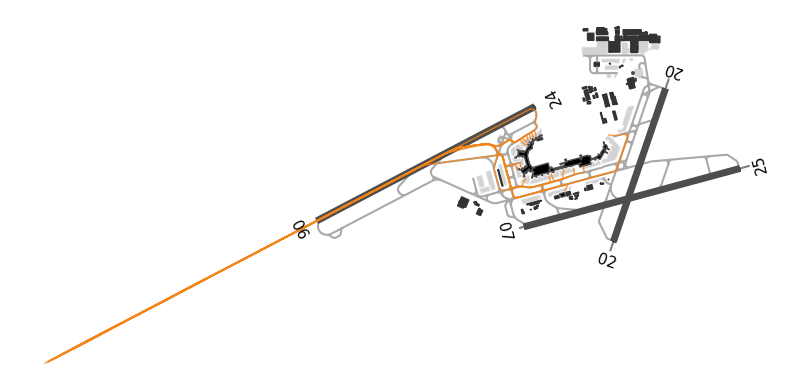
take the last 10 minutes of trajectories landing at LFPO (similar to above):
t1 = ( quickstart .has("landing('LFPO')") .last('10 min') .eval(max_workers=4) ) with plt.style.context('traffic'): fig, ax = plt.subplots(subplot_kw=dict(projection=Lambert93())) t1.plot(ax, color="#f58518") airports['LFPO'].plot( ax, footprint=False, runways=dict(linewidth=1, color='black', zorder=3) ) ax.spines['geo'].set_visible(False)

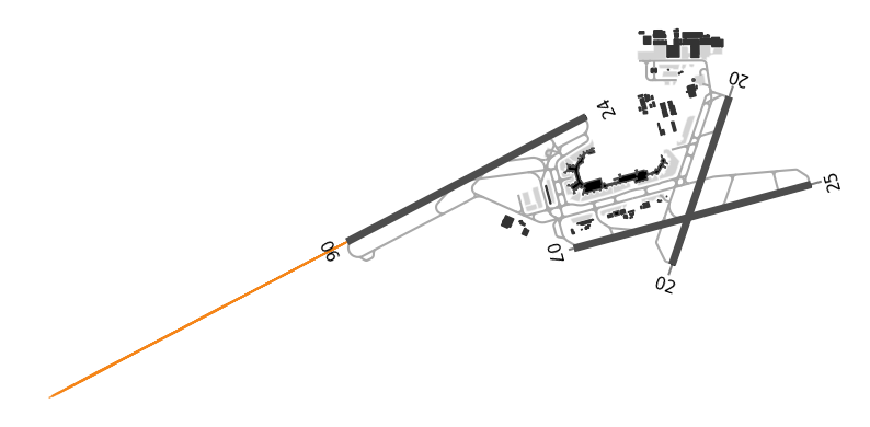
take the last minute of the segment of trajectory which is aligned on runway 06:
t2 = ( quickstart .next('landing("LFPO")') .query("ILS == '06'") .last("1 min") .eval(max_workers=4) ) with plt.style.context('traffic'): fig, ax = plt.subplots(subplot_kw=dict(projection=Lambert93())) t2.plot(ax, color="#f58518") airports['LFPO'].plot(ax, labels=dict(fontsize=11)) ax.spines['geo'].set_visible(False)
select full trajectories landing on runway 06 from one minute before landing:
import pandas as pd def last_minute_with_taxi(flight: "Flight") -> "None | Flight": for segment in flight.landing("LFPO"): if segment.ILS_max == "06": return flight.after(segment.stop - pd.Timedelta("1 min")) t3 = quickstart.iterate_lazy().pipe(last_minute_with_taxi).eval() with plt.style.context('traffic'): fig, ax = plt.subplots(subplot_kw=dict(projection=Lambert93())) t3.plot(ax, color="#f58518", zorder=3) airports['LFPO'].plot(ax, labels=dict(fontsize=11)) ax.spines['geo'].set_visible(False)
select trajectories with more than one runway alignment at LFPG:
def more_than_one_alignment(flight: "Flight") -> "None | Flight": segments = flight.landing("LFPG") if first := next(segments, None): if second := next(segments, None): return flight.after(first.start - pd.Timedelta('90s')) t4 = quickstart.iterate_lazy().pipe(more_than_one_alignment).eval() flight = t4[0] segments = flight.landing("LFPG") first = next(segments) forward = first.first("70s").forward(minutes=4) chart = ( alt.layer( airports["LFPG"].geoencode( footprint=False, runways=dict(strokeWidth=1), labels=dict(fontSize=10), ), flight.geoencode().mark_line(stroke="#bab0ac"), forward.geoencode(stroke="#79706e", strokeDash=[7, 3], strokeWidth=0.8), first.geoencode().encode(alt.Color("ILS")), next(segments).geoencode().encode(alt.Color("ILS")), ) .properties( title=f"Runway change at LFPG airport with {flight.callsign}", width=600, ) .configure_view(stroke=None) .configure_legend(orient="bottom") .configure_title(font="Lato", fontSize=16, anchor="start") ) chart