Quantitative Assessments of Runway Excursion Precursors using Mode S data
Xavier Olive, Pierre Bieber
Data preparation
The dataset consists of one month of trajectories around Toulouse airport. The first step is to isolate trajectories landing. The following code is a suggestion to select such trajectories.
from tqdm.autonotebook import tqdm
from typing import List
from traffic.core import Traffic, Flight

february = Traffic.from_file("data/lfbo_february.pkl.gz")

cumul: List[Flight] = []

# The first step is to assign a specific id to all trajectories
for item in tqdm(february.assign_id()):

    flight = (
        item
        # remove samples with no positional data
        .query("latitude == latitude")
        # default median filters
        .filter()
    )

    # remove trajectories with not enough samples
    if len(item) < 100:
        continue

    # Keep flights landing at LFBO
    guess = flight.guess_landing_airport()
    if guess.airport.icao != "LFBO" or guess.distance > 6000:
        continue

    cumul.append(flight)

t_landing = Traffic.from_flights(cumul)

# backup
# t_landing.to_pickle("data/february_landing.pkl")
Since we want to focus on aircraft landing on runway 32, we need to apply a bit more filtering.
The library offers a tool trying to guess the runway on which an aircraft lands (only on major airports). The heuristics must be perfectible: warnings are raised when the assigned runway looks dodgy. We remove by hand trajectories with a raised warning (this could be automated in a better way…)
cumul: List[Flight] = []

for item in tqdm(t_landing):

    if item.icao24 in ["38413a", "380efa", "3801da", "398588"]:
        # aircraft with buggy data
        continue
    flight = item.query(
        # vertical_rate being NaN is often a sign of buggy data
        "~onground and vertical_rate == vertical_rate"
    )

    # extra sanity checks to take away invalid trajectories
    if len(flight) < 30 or flight.data.vertical_rate.mean() > -2.5:
        continue

    # only keep trajectories landing on runway 32
    runway = flight.guess_landing_runway()
    if runway.name.startswith("32"):
        cumul.append(
            flight.between(runway.point.start, runway.point.stop)
        )

# We remove the following id because the runway detection seems to have failed
t_32 = Traffic.from_flights(
    f for f in final if f.flight_id !='AIB103_1754'
)

# backup
# t_32.to_pickle("data/february_landing_32.pkl")

t_32
WARNING:root:(AF118VA_2073) Candidate runway 14L is not consistent with average track 323.0394445508367.
WARNING:root:(AIB103_1754) Candidate runway 32L is not consistent with average track 142.5683970215894.
WARNING:root:(AIB1776_555) Candidate runway 14L is not consistent with average track 180.0.
[...]
| count | |
|---|---|
| flight_id | |
| AAF733P_3907 | 598 |
| DLH57A_353 | 598 |
| DLH53U_4609 | 598 |
| DLH53U_4660 | 598 |
| DLH53U_4708 | 598 |
| DLH53U_4709 | 598 |
| DLH57A_320 | 598 |
| DLH57A_323 | 598 |
| DLH57A_333 | 598 |
| DLH57A_336 | 598 |
We end up with a dataset of 1361 trajectories landing at Toulouse airport in February 2017 on QFU32.
However, trimming trajectories to final approaches requires a bit more work. We use here navigational beacons in the official procedures. Only main navaids are provided by the data source embedded in the library: we add the coordinates manually and automate some plotting for following figures.
from traffic.core.mixins import PointMixin


class Point(PointMixin):
    """This mixin provides the interface to plot the elements on maps."""

    def __init__(self, lat, lon, name):
        self.latitude = lat
        self.longitude = lon
        self.name = name


# Coordinates for key positions for final approach in LFBO
procedure_points = {
    "BO310": Point(lat=43.787917, lon=1.200389, name="BO310"),
    "BO410": Point(lat=43.465222, lon=1.536195, name="BO410"),
    "BO510": Point(lat=43.794389, lon=1.188889, name="BO510"),
    "BO610": Point(lat=43.468472, lon=1.528195, name="BO610"),
    "14L": Point(lat=43.6374315, lon=1.3575536, name="14L"),
    "14R": Point(lat=43.6446126, lon=1.3454186, name="14R"),
    "32L": Point(lat=43.6185805, lon=1.3725227, name="32L"),
    "32R": Point(lat=43.6156582, lon=1.3802184, name="32R"),
}


def params(point_id):
    left_side = point_id in ["BO610", "32L"]
    return dict(
        shift=dict(units="dots", x=-15 if left_side else 15),
        text_kw=dict(
            s=point_id,
            horizontalalignment="right" if left_side else "left",
            bbox=dict(facecolor="sandybrown", alpha=0.5, boxstyle="round"),
        ),
    )


def plot_points(ax):
    for point_id in ["BO610", "BO410", "32L", "32R"]:
        value = procedure_points[point_id]
        value.plot(ax, s=7, zorder=2, **(params(point_id)))
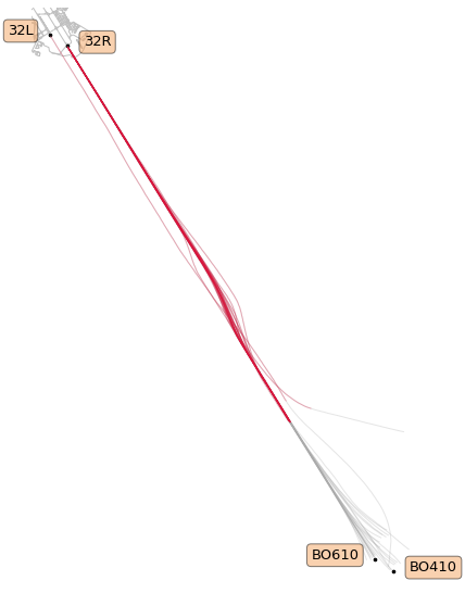
With the following map, we can position trajectories landing on QFU32 with respect to the above mentioned navigational beacons.
from cartopy.crs import EuroPP
from traffic.data import airports

with plt.style.context('traffic'):
    fig, ax = plt.subplots(
        subplot_kw=dict(projection=EuroPP())
    )

    airports['LFBO'].plot(ax)
    plot_points(ax)

    t_32.plot(ax, alpha=.3, zorder=-2)

    ax.spines['geo'].set_visible(False)
    ax.background_patch.set_visible(False)
First visual check: so far so good! Some trajectories seem to have their positions quite drifted.
In order to select the final approach, we trim the trajectories between their closest timestamp near one of the BOx10 beacon, and near one of the two runway thresholds. We filter trajectories passing too far away from this beacons in order to get rid of trajectories seeming to have a wrong estimation of their position (probable drifting of the inertial navigation system). We eliminate a few more trajectories but consider it still acceptable for a statistical analysis.
from typing import Any, Dict, List

import pandas as pd
from pitot import geodesy


cumul: List[Dict[str, Any]] = []

for flight in tqdm(t_32):
    bo = flight.closest_point([proc["BO610"], proc["BO410"]])
    rw = flight.closest_point([proc["32L"], proc["32R"]])
    cumul.append(
        dict(
            flight_id=flight.flight_id,
            # estimation of roll-out point (closest to BOx10)
            bo=bo.name,
            bo_ts=bo.point.timestamp,
            bo_d=bo.distance,
            # time at runway threshold
            rw=rw.name,
            rw_ts=rw.point.timestamp,
            rw_d=rw.distance,
        )
    )

analysis = pd.DataFrame.from_records(cumul)

# backup
# analysis.to_pickle("analysis.pkl")

t_final = Traffic.from_flights(
    t_32[line.flight_id]
    # trim the trajectory to final approach
    .between(line.bo_ts, line.rw_ts)
    # add one column for distance to the proper runway threshold
    .assign(
        distance=lambda df: geodesy.distance(
            df.latitude.values,
            df.longitude.values,
            df.shape[0] * [procedure_points[line.rw].latitude],
            df.shape[0] * [procedure_points[line.rw].longitude],
        )
    )
    # this last filtering removes flight with data which is erroneous or
    # irrelevant to our current case study.
    for _, line in analysis.query("rw_d < 400 and bo_d < 5000").iterrows()
)

# backup
# t_final.to_pickle("data/february_landing_32_final.pkl")

t_final
| count | |
|---|---|
| flight_id | |
| BGA191A_2873 | 374 |
| BGA241B_2939 | 371 |
| BGA251B_2940 | 349 |
| HOP41FK_4016 | 348 |
| GAF612_4783 | 347 |
| HOP17VJ_4101 | 347 |
| HOP11VJ_4053 | 342 |
| N721EE_7072 | 341 |
| AIB07EO_1779 | 337 |
| BGA121D_3023 | 336 |
import matplotlib.pyplot as plt

from cartopy.crs import EuroPP
from traffic.data import airports
from traffic.visualize import rivers

with plt.style.context('traffic'):
    fig, ax = plt.subplots(
        subplot_kw=dict(projection=EuroPP())
    )

    airports['LFBO'].plot(ax)
    plot_points(ax)

    t_final.plot(ax, alpha=.3,)
    t_final.query('distance < 8 * 1852').plot(ax, color='crimson', alpha=.3,)

    ax.spines['geo'].set_visible(False)
    ax.background_patch.set_visible(False)
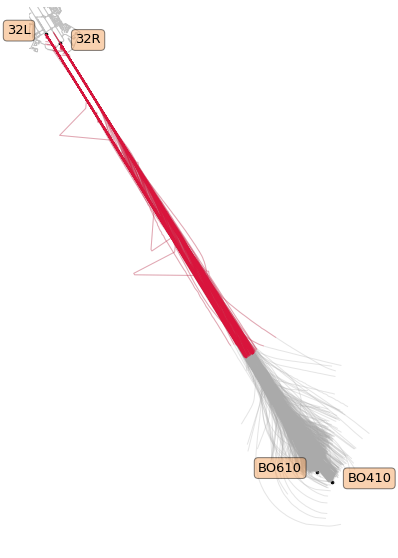
Visual check: in the paper we consider the final 8 nautical miles (in red).
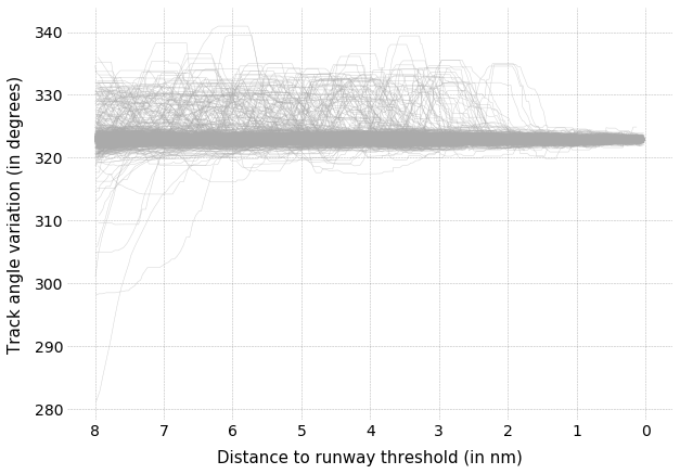
For the following, the idea is to consider all track angle signals and to analyse their modes of variation. Here is the full dataset plotted.
with plt.style.context('traffic'):
    fig, ax = plt.subplots(figsize=(10, 7))
    ax.invert_xaxis()

    ax.set_xlabel("Distance to runway threshold (in nm)", labelpad=10, fontsize=15)
    ax.set_ylabel("Track angle variation (in degrees)", labelpad=10, fontsize=15)

    for flight in t_final.query('distance < 8*1852'):
        ax.plot(
            flight.data.distance/1852,
            flight.data.heading,
            color='#aaaaaa',
            alpha=.5,
            linewidth=.5
        )
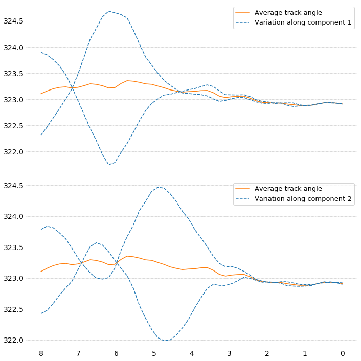
Functional Principal Component Analysis
We resample all trajectories to 50 points and fit a (functional) PCA on the dataset. The following plot displays some modes of variation around the average signal.
import numpy as np
from sklearn.decomposition import PCA

# Prepare a dataset of track angles on final approach
X = np.vstack(
    [
        # for this demonstration we take 50 samples on final approach
        flight.resample(50).data.track
        for flight in t_final.query("distance < 8*1852")
    ]
)

# keep track of the identifier for each trajectory
flight_ids = list(flight.flight_id for flight in t_final)

pca = PCA()
X_t = pca.fit_transform(X)
with plt.style.context("traffic"):

    fig, ax = plt.subplots(2, 1, figsize=(10, 10), sharex=True)
    xlim = np.linspace(8, 0, 50)

    m_theme = dict(linestyle='solid', color='#ff7f0e')
    v_theme = dict(linestyle="--", color="#1f77b4")

    for i, a in enumerate(ax):

        var_i = np.sqrt(pca.explained_variance_[i + 1])
        theta_i = pca.components_[i + 1]

        a.plot(xlim, pca.mean_, **m_theme,
               label="Average track angle")
        a.plot(xlim, pca.mean_ + var_i * theta_i, **v_theme,
               label=f"Variation along component {i+1}")
        a.plot(xlim, pca.mean_ - var_i * theta_i, **v_theme)

        a.legend()

    a.invert_xaxis()
    fig.tight_layout()
One of the main ideas of the paper was to specifically select trajectories with strong components along these modes of variation. It appears they follow a specific pattern of late runway changes.
second_component = np.abs(X_t[:, 1])
selected_flights = Traffic.from_flights(
    t_final[flight_id]
    for flight_id, component in zip(flight_ids, second_component)
    if component > np.percentile(second_component, 98)
)
from cartopy.crs import EuroPP
from traffic.data import airports
from traffic.visualize import rivers

with plt.style.context('traffic'):
    fig, ax = plt.subplots(
        subplot_kw=dict(projection=EuroPP())
    )

    airports['LFBO'].plot(ax)
    plot_points(ax)

    selected_flights.plot(ax, color='#aaaaaa', alpha=.3)
    selected_flights.query('distance < 8 * 1852').plot(
        ax, color='crimson', alpha=.3
    )

    ax.spines['geo'].set_visible(False)
    ax.background_patch.set_visible(False)