How to access airspace information?
Each Air Control Center (ACC), in charge of providing air traffic control services to controlled flights within its airspace, is subdivided into elementary sectors that are used or combined to build control sectors operated by a pair of air traffic controllers.
Airspace sectorisation consists in partitioning the overall ACC airspace into a given number of these control sectors. In most centres, the set of control sectors deployed, i.e. the sector configuration, varies throughout the day. Basically, sectors are split when controllers’ workload increases, and merged when it decreases.
An Airspace is represented as a set of polygons of geographical coordinates, extruded to a lower and upper altitudes. Airspaces can be of different types, corresponding to different kinds of activities allowed (civil, military, glider, etc.) or services provided.
- a Flight Information Region (FIR) is the largest regular division of airspace in use in the world today, roughly corresponding to a country, although some FIRs encompass several countries, and larger countries are subdivided into a number of regional FIRs.Read more about FIRs of the world
- a Terminal Maneuvering Area (TMA) is usually controlled by the airport it is attached to: this airspace is usually reserved for aircraft landing at or taking off from that airport;
- an Air Route Traffic Control Center (ARTCC) or an Air Control Center (ACC) represents the area that is controlled by people located in the same center;
- an elementary sector is usually the smallest subdivision of airspace that can be controlled by a pair of air traffic controllers.
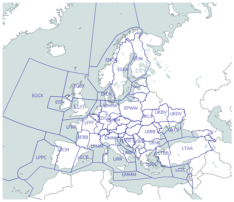
FIRs from countries in the EUROCONTROL area
Airspaces are usually handled as a wrapper around GeoDataFrame, i.e. Pandas data frames with a particular geometry feature.
from traffic.data import eurofirs

eurofirs.head()
| geometry | designator | name | type | upper | lower | latitude | longitude | |
|---|---|---|---|---|---|---|---|---|
| 0 | POLYGON ((6.19247 49.96404, 6.19404 49.96043, ... | EBBU | BRUSSELS FIR | FIR | 195.0 | 0.0 | 50.628406 | 4.600560 |
| 1 | POLYGON ((6.9056 45.67116, 6.90687 45.67508, 6... | LIMM | MILANO FIR | FIR | 195.0 | 0.0 | 45.030624 | 10.499386 |
| 2 | POLYGON ((6.12122 46.25472, 6.12454 46.25131, ... | LFMM | MARSEILLE FIR | FIR | 195.0 | 0.0 | 42.845677 | 5.925558 |
| 3 | POLYGON ((-13 45, -13 43, -15 42, -15 36.5, -1... | LPPO | SANTA MARIA OCEANIC FIR | FIR | inf | 0.0 | 34.190600 | -29.363399 |
| 4 | POLYGON ((30.56583 51.30833, 30.56722 51.31389... | UKBV | KYIV FIR | FIR | 275.0 | 0.0 | 50.086590 | 30.888969 |
As FIRs usually consist of a single polygon with an upper and a lower limit (in Flight Level, i.e. FL 300 corresponds to 30,000 ft), their representation is simple in a Jupyter environment.
eurofirs["ENOB"]
- lower: 0 | upper: inf
Leaflet representations are also easily accessible:
eurofirs["EKDK"].map_leaflet()
The following snippet plots the whole dataset:
import matplotlib.pyplot as plt

from cartes.crs import LambertConformal
from cartes.utils.features import countries, lakes, ocean

fig, ax = plt.subplots(
    figsize=(15, 10),
    subplot_kw=dict(projection=LambertConformal(10, 45)),
)

ax.set_extent((-20, 45, 25, 75))

ax.add_feature(countries(scale="50m"))
ax.add_feature(lakes(scale="50m"))
ax.add_feature(ocean(scale="50m"))

ax.spines['geo'].set_visible(False)

for fir in eurofirs:
    fir.plot(ax, edgecolor="#3a3aaa")
    if fir.designator not in ["ENOB", "LPPO", "GCCC"] and fir.area > 1e11:
        fir.annotate(
            ax,
            s=fir.designator,
            ha="center",
            color="#3a3aaa",
            fontname="Ubuntu",
            fontsize=13,
        )
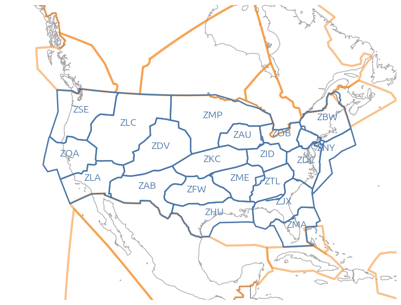
FIRs and ARTCC from the FAA
The Federal Aviation Administration (FAA) publishes some data about their airspace in open data. The data is automatically downloaded the first time you try to access it.
Find more about this service here. On the following map, Air Route Traffic Control Centers (ARTCC) are displayed together with neighbouring FIRs.
from traffic.data.faa import airspace_boundary
import matplotlib.pyplot as plt

from cartes.crs import AzimuthalEquidistant
from cartes.utils.features import countries

fig, ax = plt.subplots(
    figsize=(10, 10),
    subplot_kw=dict(projection=AzimuthalEquidistant(central_longitude=-100)),
)

ax.add_feature(countries(scale="50m"))
ax.set_extent((-130, -65, 15, 60))
ax.spines['geo'].set_visible(False)


for airspace in airspace_boundary.query(
    'type == "FIR" and designator.str[0] in ["C", "M", "T"]'
):
    airspace.plot(ax, edgecolor="#f58518", lw=3, alpha=0.5)

for airspace in airspace_boundary.query(
    'type == "ARTCC" and designator != "ZAN"'  # Anchorage
).at_level(100):
    airspace.plot(ax, edgecolor="#4c78a8", lw=2)
    airspace.annotate(
        ax,
        s=airspace.designator,
        color="#4c78a8",
        ha="center",
        fontname="Ubuntu",
        fontsize=14,
    )
Airspace data from EUROCONTROL
Warning
Access conditions and configuration for these sources of data is detailed here.
Tip
According to the source of data you may have access to, different parsers are
implemented but they expose the same API. Data is usually not exactly
consistent (coordinates, types, etc.) but you should still be able to safely
replace nm_airspaces with aixm_airspaces in the following examples.
from traffic.data import nm_airspaces
Get a single airspace
In these files, airspaces being a composition of elementary airspaces are widespread. Their union is computed and yields a list of polygons associated with minimum and maximum flight levels.
nm_airspaces["EDYYUTAX"]
- lower: 245 | upper: 255
- lower: 255 | upper: 295
- lower: 295 | upper: inf
The Leaflet view and the Matplotlib view, flatten the polygon prior to displaying it:
nm_airspaces["EDYYUTAX"].map_leaflet()
Get many airspaces
Airspaces are stored as a GeoDataFrame, so all pandas operators may be applied to get a subset of them, for example based on their types or designator.
All available airspace types can be accessed here:
nm_airspaces.data["type"].unique()
array(['AREA', 'FIR', 'NAS', 'AUAG', 'CS', 'ES', 'AUA', 'REG', 'CRSA',
       'ERSA', 'CRAS', 'ERAS', 'CLUS'], dtype=object)
In the following examples, we get all FIR spaces in the LF domain (France). You
may notice that a single designator may be represented by several entries in the
GeoDataFrame, but the representation of each shape you get through iteration,
indexation or __geo_interface__ attribute (used in Altair) is properly
computed.
france_fir = nm_airspaces.query('type == "FIR" and designator.str.startswith("LF")')
france_fir.head(10)
| designator | component | name | type | geometry | upper | lower | |
|---|---|---|---|---|---|---|---|
| 218607 | LFBBFIR | LFBBFIR | NaN | FIR | POLYGON ((2.83333 46.75, 2.83778 46.72917, 2.8... | 195.0 | 0.0 |
| 218615 | LFEEFIR | LFEEFIR | NaN | FIR | POLYGON ((6.00944 46.54361, 6.1325 46.58305, 6... | 195.0 | 0.0 |
| 218616 | LFEEFIR | LFEEFIR | NaN | FIR | POLYGON ((6.71667 47.05333, 6.64167 47.02444, ... | 195.0 | 0.0 |
| 218617 | LFEEFIR | LFEEFIR | NaN | FIR | POLYGON ((5.99917 46.99861, 6.02639 46.98417, ... | 195.0 | 0.0 |
| 218618 | LFEEFIR | LFEEFIR | NaN | FIR | POLYGON ((5.18333 46.7, 5.33333 46.7, 5.35 46.... | 195.0 | 0.0 |
| 218619 | LFEEFIR | LFEEFIR | NaN | FIR | POLYGON ((6.39667 46.78222, 6.39167 46.74333, ... | 195.0 | 0.0 |
| 218620 | LFEEFIR | LFEEFIR | NaN | FIR | POLYGON ((6.39667 46.78222, 6.44139 46.76, 6.4... | 195.0 | 0.0 |
| 218621 | LFEEFIR | LFEEFIR | NaN | FIR | POLYGON ((6 49.45556, 6.05556 49.46667, 6.115 ... | 195.0 | 0.0 |
| 218626 | LFFFFIR | LFFFFIR | NaN | FIR | POLYGON ((2 51.11667, 2.245 51.10139, 2.55 51.... | 195.0 | 0.0 |
| 218627 | LFFFFIR | LFFFFIR | NaN | FIR | POLYGON ((2.81667 49.15, 6 49.45556, 5.825 49.... | 195.0 | 0.0 |
import altair as alt

from cartes.atlas import europe

france = alt.Chart(europe.topo_feature).transform_filter(
    "datum.properties.geounit == 'France'"
)

base = (
    alt.Chart(france_fir)
    .mark_geoshape(stroke="white")
    # In this dataset, UIR and FIR are both tagged as FIR
    # => we reconstruct the type and designator
    .transform_calculate(suffix="slice(datum.designator, -3)")
    .transform_calculate(designator="slice(datum.designator, 0, -3)")
    .properties(width=300)
)

chart = (
    alt.concat(
        alt.layer(
            base.encode(alt.Color("designator:N", title="FIR"))
            .transform_filter("datum.suffix == 'FIR'"),
            france.mark_geoshape(stroke="#ffffff", strokeWidth=3, fill="#ffffff00"),
            france.mark_geoshape(stroke="#79706e", strokeWidth=1, fill="#ffffff00"),
            base.mark_text(fontSize=14, font="Lato")
            .encode(
                alt.Latitude("latitude:Q"),
                alt.Longitude("longitude:Q"),
                alt.Text("designator:N"),
            )
            .transform_filter("datum.suffix == 'FIR'"),
        ),
        alt.layer(
            base.encode(alt.Color("designator:N"))
            .transform_filter("datum.suffix == 'UIR'"),
            france.mark_geoshape(stroke="#ffffff", strokeWidth=3, fill="#ffffff00"),
            france.mark_geoshape(stroke="#79706e", strokeWidth=1, fill="#ffffff00"),
        )
    )
    .configure_legend(orient="bottom", labelFontSize=12, titleFontSize=12)
    .configure_view(stroke=None)
)

chart
Warning
Note that the FIR and UIR boundaries do not presume anything about how air traffic control is organised in that area. See below a map of the areas controlled by different en-route air traffic control centres in France.
centres = ["LFBBBDX", "LFRRBREST", "LFEERMS", "LFFFPARIS", "LFMMRAW", "LFMMRAE"]
subset = (
    nm_airspaces.query(f"designator in {centres}")
    .replace("LFMMRAW", "Aix-en-Provence (Sud-Est)")
    .replace("LFMMRAE", "Aix-en-Provence (Sud-Est)")
    .replace("LFBBBDX", "Bordeaux (Sud-Ouest)")
    .replace("LFEERMS", "Reims (Est)")
    .replace("LFFFPARIS", "Athis-Mons (Nord)")
    .replace("LFRRBREST", "Brest (Ouest)")
)


chart = (
    alt.hconcat(
        alt.layer(
            alt.Chart(subset.at_level(220))
            .mark_geoshape(stroke="white")
            .encode(
                alt.Tooltip(["designator:N"]),
                alt.Color("designator:N", title="CRNA"),
            ),
            france.mark_geoshape(stroke="#ffffff", strokeWidth=3, fill="#ffffff00"),
            france.mark_geoshape(stroke="#79706e", strokeWidth=1, fill="#ffffff00"),
        ).properties(title="FL 220", width=300),
        alt.layer(
            alt.Chart(subset.at_level(320))
            .mark_geoshape(stroke="white")
            .encode(
                alt.Tooltip(["designator:N"]),
                alt.Color("designator:N", title="CRNA"),
            ),
            france.mark_geoshape(stroke="#ffffff", strokeWidth=3, fill="#ffffff00"),
            france.mark_geoshape(stroke="#79706e", strokeWidth=1, fill="#ffffff00"),
        ).properties(title="FL320", width=300),
    )
    .configure_legend(orient="bottom", labelFontSize=12, titleFontSize=12)
    .configure_view(stroke=None)
    .configure_title(fontSize=16, font="Lato", anchor="start")
)

chart
Iterate through many airspaces
The following trick lets you return the largest CS sector with a designator starting with LFBB (Bordeaux FIR/ACC).
# Find the largest CS in Bordeaux ACC
from operator import attrgetter

max(
    nm_airspaces.query('type == "CS" and designator.str.startswith("LFBB")'),
    key=attrgetter("area"),  # equivalent to `lambda x: x.area`
)
- lower: 145 | upper: 195
- lower: 195 | upper: 265
- lower: 265 | upper: inf
Free Route Areas (FRA) from EUROCONTROL
The Free Route information consists of regular airspace information:
from traffic.data import nm_freeroute
nm_freeroute
| geometry | designator | upper | lower | name | type | |
|---|---|---|---|---|---|---|
| 0 | POLYGON ((27.69944 51.47972, 26.79833 51.76639... | BEL_FRA | 660.0 | 275.0 | FRA | |
| 1 | POLYGON ((-39 63.5, -34.25089 65.70462, -28.65... | BIRD_DOMESTIC | 660.0 | 0.0 | FRA | |
| 2 | POLYGON ((0.00039 63.01636, 5e-5 72.99989, 0 8... | BODO_OCEANIC | 660.0 | 0.0 | FRA | |
| 3 | POLYGON ((18.06361 56.11861, 18.01861 56.09528... | BOREALIS | 660.0 | 285.0 | FRA | |
| 4 | POLYGON ((21 59, 20.91583 59.04783, 20.818 59.... | BOREALIS | 660.0 | 95.0 | FRA | |
| ... | ... | ... | ... | ... | ... | ... |
| 63 | POLYGON ((30.53333 43.68333, 29.03333 43.73333... | SEE_FRA_SOUTH | 660.0 | 105.0 | FRA | |
| 64 | POLYGON ((-60 65, -59.97538 60.00695, -60.4253... | SONDRESTROM | 660.0 | 0.0 | FRA | |
| 65 | POLYGON ((29.68778 48.06472, 29.88445 48.19139... | UKOV_FRA | 660.0 | 275.0 | FRA | |
| 66 | POLYGON ((27.85 49.76167, 27.04389 50.18195, 2... | UKRNESFRA | 660.0 | 275.0 | FRA | |
| 67 | POLYGON ((25.7775 47.94056, 25.71667 47.93222,... | UKRNESFRA | 660.0 | 275.0 | FRA |
68 rows × 6 columns
nm_freeroute["BOREALIS"].map_leaflet(zoom=3)
However, in addition to these airspace, there is a database of points attached to a Free Route Area:
Irefer to I ntermediate points in the middle of an airspace;EandXmark points of E ntry and e X it;AandDrefer to A rrival and D eparture and are attached to an airport.
nm_freeroute.points.query('FRA == "BOREALIS"')
| FRA | type | name | latitude | longitude | airport | |
|---|---|---|---|---|---|---|
| 5 | BOREALIS | I | TUSRU | 59.000000 | 6.266667 | NaN |
| 6 | BOREALIS | I | EVGUN | 58.266667 | 10.000000 | NaN |
| 7 | BOREALIS | EX | EVGUN | 58.266667 | 10.000000 | NaN |
| 37 | BOREALIS | I | VEKAB | 70.250000 | 29.216667 | NaN |
| 41 | BOREALIS | I | NENLA | 61.166667 | 9.333333 | NaN |
| ... | ... | ... | ... | ... | ... | ... |
| 2493 | BOREALIS | D | OLNOP | 66.188611 | 24.705278 | EFRO |
| 2496 | BOREALIS | D | ARMUV | 59.140278 | 23.466944 | EEKA |
| 2508 | BOREALIS | D | SALLO | 54.916667 | 13.386111 | EKCH |
| 2508 | BOREALIS | D | SALLO | 54.916667 | 13.386111 | EKRK |
| 2508 | BOREALIS | D | SALLO | 54.916667 | 13.386111 | ESMS |
2399 rows × 6 columns