Calibration flights with SAVAN trajectories
There are 86 VOR and VOR-DME installations in France and these must all be recalibrated on a yearly basis. Recently, there has been an effort to reduce the number of calibration flights, and ad hoc trajectories have been designed to cover the 360° range around all VOR installations with a reduced number of trajectories.
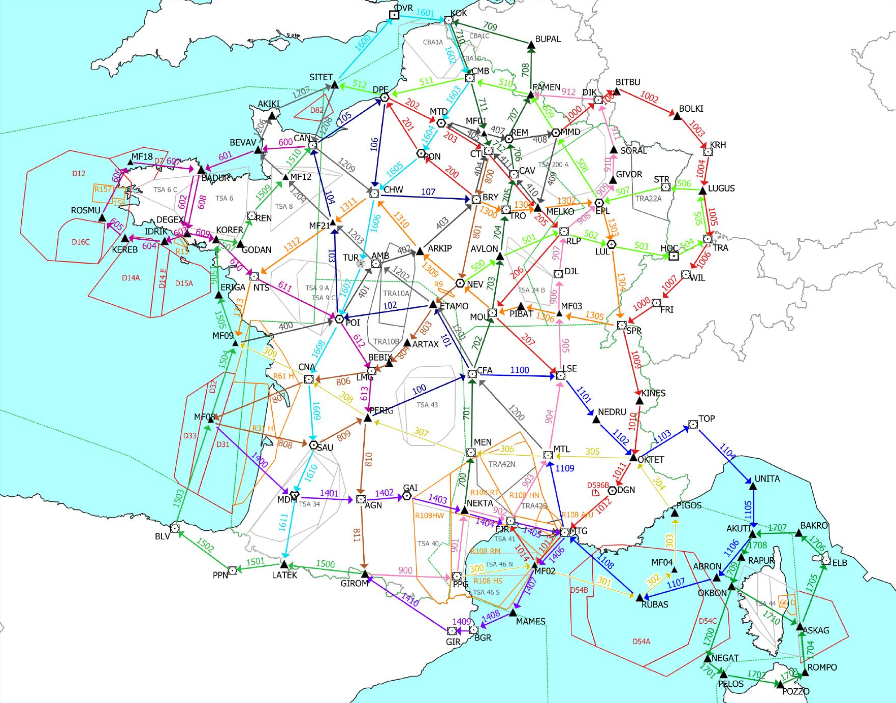
As a result, every year in France, 17 trajectories are flown to cover and calibrate all the VOR installations, according to the map below.
Those trajectories are tagged as SAVAN, which stands for Système Automatique de Vérification en vol des Aides à la Navigation aérienne (Automatic system for in-flight calibration for navigational aids)
# Trajectories flown in 2021 are provided in the following dataset, limited
# to the coverage of the OpenSky Network.

from traffic.data.samples import savan

savan.summary(['icao24', 'callsign', 'start', 'stop']).eval()
| icao24 | callsign | start | stop | |
|---|---|---|---|---|
| 0 | 39b415 | SAVAN01 | 2022-03-21 08:33:04+00:00 | 2022-03-21 11:50:02+00:00 |
| 1 | 39b415 | SAVAN02 | 2022-03-21 14:33:59+00:00 | 2022-03-21 17:45:50+00:00 |
| 2 | 39b415 | SAVAN03 | 2022-03-22 07:32:27+00:00 | 2022-03-22 10:53:27+00:00 |
| 3 | 39b415 | SAVAN04 | 2022-03-22 12:53:47+00:00 | 2022-03-22 15:59:59+00:00 |
| 4 | 39b415 | SAVAN05 | 2022-03-23 07:35:52+00:00 | 2022-03-23 10:41:04+00:00 |
| 5 | 39b415 | SAVAN06 | 2022-03-23 12:57:59+00:00 | 2022-03-23 15:59:59+00:00 |
| 6 | 39b415 | SAVAN07 | 2022-03-24 07:33:50+00:00 | 2022-03-24 10:38:08+00:00 |
| 7 | 39b415 | SAVAN08 | 2022-03-24 13:14:08+00:00 | 2022-03-24 16:32:06+00:00 |
| 8 | 39b415 | SAVAN09 | 2022-03-25 07:34:52+00:00 | 2022-03-25 10:38:52+00:00 |
| 9 | 39b415 | SAVAN10 | 2022-03-25 13:03:05+00:00 | 2022-03-25 16:45:30+00:00 |
| 10 | 39b415 | SAVAN11 | 2022-03-28 06:35:38+00:00 | 2022-03-28 10:17:46+00:00 |
| 11 | 39b415 | SAVAN12 | 2022-03-28 12:12:29+00:00 | 2022-03-28 15:18:29+00:00 |
| 12 | 39b415 | SAVAN13 | 2022-03-29 06:39:30+00:00 | 2022-03-29 09:55:54+00:00 |
| 13 | 39b415 | SAVAN14 | 2022-03-29 12:01:33+00:00 | 2022-03-29 15:29:04+00:00 |
| 14 | 39b415 | SAVAN15 | 2022-04-15 06:31:37+00:00 | 2022-04-15 09:20:59+00:00 |
| 15 | 39b415 | SAVAN16 | 2022-04-15 12:04:11+00:00 | 2022-04-15 15:21:06+00:00 |
| 16 | 39b415 | SAVAN17 | 2022-03-16 09:03:05+00:00 | 2022-03-16 09:47:50+00:00 |
| 17 | 39b415 | SAVAN17 | 2022-03-16 10:14:30+00:00 | 2022-03-16 11:32:52+00:00 |
Trajectories can be considered individually:
savan['SAVAN01'].map_leaflet(zoom=5)
But it makes more sense to plot them all together. The following cells detail how we come to the full map below:
savan['SAVAN01'].simplify(1e3).geoencode()
import altair as alt

alt.layer(
    savan['SAVAN01'].simplify(1e3).geoencode(),
    savan['SAVAN02'].simplify(1e3).geoencode()
)
alt.layer(
    savan['SAVAN01'].simplify(1e3).geoencode().encode(alt.Color('callsign')),
    savan['SAVAN02'].simplify(1e3).geoencode().encode(alt.Color('callsign'))
)
alt.layer(
    # the * operator serves as list unpacking
    *(flight.simplify(1e3).geoencode().encode(alt.Color('callsign')) for flight in savan)
)
The cartes package helps providing layouts for better maps.
from cartes.atlas import france
from cartes.crs import Lambert93

chart = (
   alt.layer(
      alt.Chart(france.topo_feature)
      .mark_geoshape(fill="None", stroke="#bab0ac")
      .project(**Lambert93()),
      # the * operator serves as list unpacking
      *(flight.simplify(1e3).geoencode().encode(alt.Color('callsign')) for flight in savan)
   )
   .properties(width=600, height=600)
   .configure_view(stroke=None)
   .configure_legend(orient='bottom', columns=5)
)
chart
The next step for a proper visualisation is to include the VOR locations on the map. A naive approach would be to use the bounding box of “France métropolitaine” (the adjective helps excluding overseas territories with the OpenStreetMap Nominatim service.)
from traffic.data import navaids

vors = navaids.extent('France métropolitaine').query('type == "VOR"')
vors
| name | type | latitude | longitude | altitude | frequency | magnetic_variation | description | |
|---|---|---|---|---|---|---|---|---|
| 272141 | ABB | VOR | 50.135139 | 1.854694 | 220.0 | 108.45 | -1.0 | ABBEVILLE VOR-DME |
| 272179 | AFI | VOR | 50.907778 | 4.138889 | 291.0 | 114.90 | 0.0 | AFFLIGEM VOR-DME |
| 272184 | AGN | VOR | 43.888028 | 0.872861 | 896.0 | 114.80 | 0.0 | AGEN VOR-DME |
| 272196 | AJO | VOR | 41.770528 | 8.774667 | 2142.0 | 114.80 | 2.0 | AJACCIO VOR-DME |
| 272210 | ALB | VOR | 44.048167 | 8.127611 | 144.0 | 116.95 | 1.0 | ALBENGA VOR-DME |
| ... | ... | ... | ... | ... | ... | ... | ... | ... |
| 275742 | WYP | VOR | 51.048353 | 7.279997 | 0.0 | 109.60 | 1.0 | WIPPER VOR |
| 275921 | ZAR | VOR | 41.657889 | -1.030861 | 886.0 | 113.00 | 0.0 | ZARAGOZA VOR-DME |
| 275942 | ZMR | VOR | 41.530194 | -5.639694 | 2067.0 | 117.10 | -2.0 | ZAMORA VOR-DME |
| 275948 | ZUE | VOR | 47.592167 | 8.817667 | 1730.0 | 110.05 | 2.0 | ZURICH EAST VOR-DME |
| 275953 | ZWN | VOR | 49.229072 | 7.417892 | 1164.0 | 114.80 | 2.0 | ZWEIBRUECKEN VOR-DME |
206 rows × 8 columns
For the time being, the filtering based on a polygon is not provided by the library, but it is not very difficult to code it directly.
from cartes.osm import Nominatim

france_shape = Nominatim.search("France métropolitaine").shape
france_shape

from shapely.geometry import Point
from traffic.data.basic.navaid import Navaids

vors = navaids.extent('France métropolitaine').query('type == "VOR"')
vors_fr = Navaids(
 vors.data.loc[
     list(france_shape.contains(Point(x.longitude, x.latitude)) for x in vors)
 ]
)
vors_fr
| name | type | latitude | longitude | altitude | frequency | magnetic_variation | description | |
|---|---|---|---|---|---|---|---|---|
| 272141 | ABB | VOR | 50.135139 | 1.854694 | 220.0 | 108.45 | -1.0 | ABBEVILLE VOR-DME |
| 272184 | AGN | VOR | 43.888028 | 0.872861 | 896.0 | 114.80 | 0.0 | AGEN VOR-DME |
| 272196 | AJO | VOR | 41.770528 | 8.774667 | 2142.0 | 114.80 | 2.0 | AJACCIO VOR-DME |
| 272230 | AMB | VOR | 47.428917 | 1.064444 | 387.0 | 113.70 | -2.0 | AMBOISE VOR-DME |
| 272246 | ANG | VOR | 47.536861 | -0.851833 | 304.0 | 113.00 | -3.0 | ANGERS VOR |
| ... | ... | ... | ... | ... | ... | ... | ... | ... |
| 275341 | TIS | VOR | 45.881833 | 3.553583 | 2000.0 | 117.50 | 1.0 | THIERS VOR-DME |
| 275389 | TOU | VOR | 43.680833 | 1.309806 | 574.0 | 117.70 | 0.0 | TOULOUSE BLAGNAC VOR-DME |
| 275424 | TRO | VOR | 48.251222 | 3.963139 | 0.0 | 116.00 | 1.0 | TROYES BARBEREY VOR |
| 275439 | TSU | VOR | 48.753722 | 2.102361 | 547.0 | 108.25 | 0.0 | TOUSSUS LE NOBLE VOR |
| 275645 | VNE | VOR | 45.556444 | 4.883417 | 0.0 | 108.20 | 1.0 | VIENNE VOR |
86 rows × 8 columns
Here comes a better map now:
base_vor = alt.Chart(vors_fr.data).mark_point().encode(
   alt.Longitude('longitude'), alt.Latitude('latitude')
)

map_chart = (
   alt.layer(
      alt.Chart(france.topo_feature)
      .mark_geoshape(fill="None", stroke="#bab0ac"),
      # the * operator serves as list unpacking
      *(flight.simplify(1e3).geoencode().encode(alt.Color('callsign')) for flight in savan),
      base_vor,
      base_vor.mark_text(dx=20).encode(alt.Text('name'))
   )
   .project(**Lambert93())
   .properties(width=600, height=600)
   .configure_view(stroke=None)
   .configure_legend(orient='bottom', columns=5)
)
map_chart
A way to dig into how VOR installations are well covered on 360 degrees by SAVAN trajectories is to compute for each VOR and for each trajectory, which legs cover which bearing angle.
from traffic.core import Traffic

coverage = Traffic.from_flights(
    savan.assign(vor=vor.name)
    .iterate_lazy()  # optional, but this line makes it clear we loop over flights
    .phases()  # compute flight phases
    .query('phase == "LEVEL" and altitude > 20000')
    .resample("15s")  # reduce the number of points
    .distance(vor)
    .bearing(vor)
    .query("20 < distance < 100")  # only keep legs within coverage
    .longer_than("10 min")
    .eval()
    # focus roughly on Corsica, but we could go for the whole set of VORs
    for vor in vors_fr.query("latitude < 47 and longitude > 7")
)
coverage.data[['callsign', 'latitude', 'longitude', 'altitude', 'distance', 'bearing', 'vor']]
| callsign | latitude | longitude | altitude | distance | bearing | vor | |
|---|---|---|---|---|---|---|---|
| 222 | SAVAN11 | 43.425339 | 8.963439 | 28000.0 | 99.609111 | 184.881527 | AJO |
| 223 | SAVAN11 | 43.405746 | 8.961139 | 28000.0 | 98.429483 | 184.879834 | AJO |
| 224 | SAVAN11 | 43.386825 | 8.958893 | 28000.0 | 97.290168 | 184.877488 | AJO |
| 225 | SAVAN11 | 43.366668 | 8.956539 | 28000.0 | 96.076578 | 184.875962 | AJO |
| 226 | SAVAN11 | 43.346977 | 8.954184 | 28000.0 | 94.890814 | 184.872965 | AJO |
| ... | ... | ... | ... | ... | ... | ... | ... |
| 204 | SAVAN17 | 42.461746 | 8.48363 | 22000.0 | 95.301403 | 325.890187 | NIZ |
| 205 | SAVAN17 | 42.45471 | 8.488727 | 22000.0 | 95.777793 | 325.923071 | NIZ |
| 206 | SAVAN17 | 42.441349 | 8.501374 | 22000.0 | 96.756319 | 325.921902 | NIZ |
| 207 | SAVAN17 | 42.424118 | 8.525765 | 22000.0 | 98.220072 | 325.752478 | NIZ |
| 208 | SAVAN17 | 42.415699 | 8.541678 | 22000.0 | 99.035897 | 325.589422 | NIZ |
4150 rows × 7 columns
We can then produce plots to check for the coverage, here limited on South-eastern France and Corsica:
chart = (
    alt.Chart(coverage.data)
    .mark_circle()
    .encode(
        alt.X(
            "bearing",
            title="Bearing angle in degree",
            scale=alt.Scale(domain=(0, 360), nice=False),
        ),
        alt.Y("vor", title="VOR name"),
    )
    .properties(width=500)
    .configure_axisY(titleY=-10, titleAnchor="start", titleAngle=0)
    .configure_axis(titleFontSize=14, labelFontSize=12)
)
chart
Some VOR are not fully covered on this map, and we can look into more details in
the following map: a part of trajectory for SAVAN17 was out of coverage of
the OpenSky Network.
map_chart.project(**(dict(Lambert93()) | dict(scale=6000, rotate=(-8, -43, 0))))
chart = (
    alt.Chart(coverage.data)
    .mark_circle()
    .encode(
        alt.X(
            "bearing",
            title="Bearing angle in degree",
            scale=alt.Scale(domain=(0, 360), nice=False),
        ),
        alt.Y("callsign", title=None),
        alt.Row("vor", title="VOR name"),
        alt.Color("callsign", legend=None),
    )
    .transform_filter("datum.vor == 'AJO' | datum.vor == 'BTA' | datum.vor == 'FGI'")
    .properties(width=500)
    .resolve_scale(y="independent")
    .configure_header(
        labelOrient="right",
        labelAngle=0,
        labelFontSize=14,
        titleOrient="right",
        titleFontSize=14,
    )
    .configure_axis(titleFontSize=14, labelFontSize=12)
)
chart