Is this a plane?
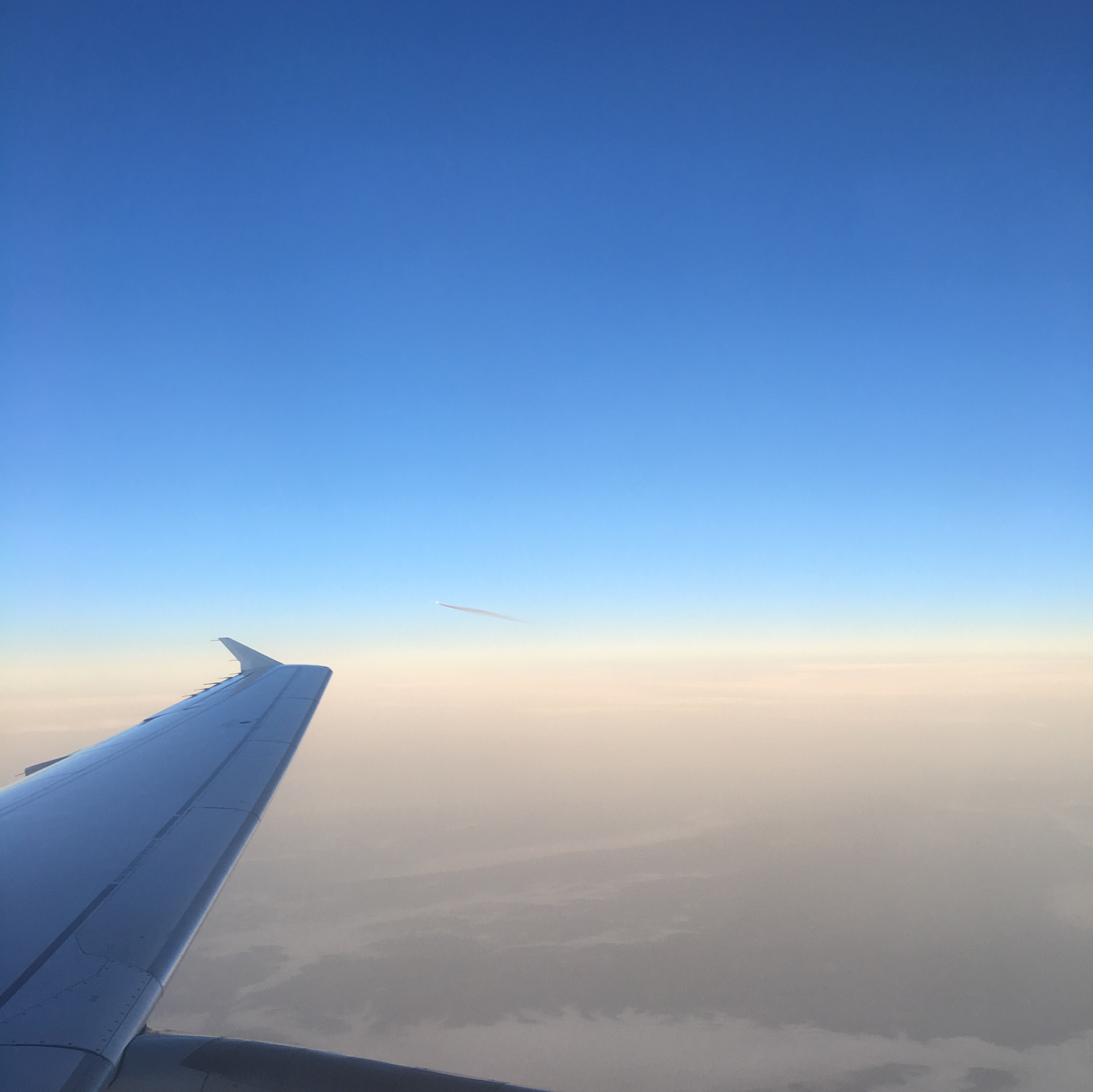
On my way to the Opensky Network workshop 2018, I could catch a picture of this aircraft which looked really close. I wondered how close it came to us considering that the usual separation rule between aircraft is of 5 nautical miles (horizontal) and 1000ft (vertical).
First let’s get information about the flight I was on.
from traffic.data import opensky

flight = opensky.history(
    "2018-11-15 06:00",  # UTC
    "2018-11-15 08:00",
    callsign='DLH07F', # of course, you need to know the callsign of your flight
    return_flight=True
)
I can check the shape of the trajectory with a good overview of Frankfurt approach up to the North.
Flight DLH07F- aircraft: 3c6608 / D-AIPH (A320)
- origin: 2018-11-15 07:16:18
- destination: 2018-11-15 08:58:38
The picture is timestamped at 06:42 UTC. Let’s have a look of what came around.
from datetime import timedelta

p = flight.at("2018-11-15 06:42")

around = opensky.history(
    p.name - timedelta(minutes=5),
    p.name + timedelta(minutes=5),
    bounds=(
        p.longitude - 0.5, p.latitude - 0.5,
        p.longitude + 0.5, p.latitude + 0.5
    )
)
around
| count | ||
|---|---|---|
| icao24 | callsign | |
| 3944ec | AFR1084 | 496 |
| 3c6608 | DLH07F | 430 |
| 406440 | EZY201G | 238 |
| 4ca816 | RYR27NB | 227 |
| 406229 | EZY71XZ | 186 |
| 495292 | TAP1245 | 184 |
| 4ca813 | RYR63TL | 181 |
| 392ae4 | HOP11JK | 133 |
| 461fa5 | FIN4YC | 45 |
| 4ca80f | RYR49ME | 9 |
It seems we get a lot of messages of this AFR1084 flight (Paris to Tunis). Let’s plot their lateral distance vs. time.
%matplotlib inline
import matplotlib.pyplot as plt

with plt.style.context('traffic'):

    fig, ax = plt.subplots(figsize=(10, 7))

    flight.distance(around['AFR1084']).plot(
        ax=ax, x='timestamp', y='lateral',
        label="Lateral distance between aircraft (in nm)"
    )
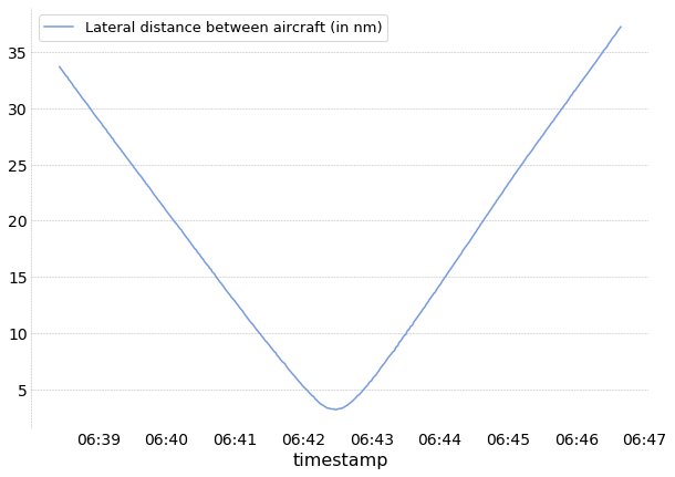
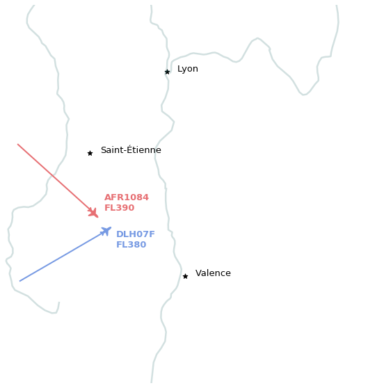
Wow, less than 5nm. We came really close! We can now plot a map, with information confirming we were properly separated (1000ft). That is only 300m of altitude difference: it really felt we were flying the same altitude though.
from cartes.crs import Lambert93
from cartes.osm import Nominatim
from cartes.utils.features import countries

from traffic.visualize.markers import rotate_marker, aircraft

with plt.style.context("traffic"):

    fig, ax = plt.subplots(subplot_kw=dict(projection=Lambert93()))

    ax.add_feature(countries())
    ax.add_feature(rivers(linewidth=2.5))
    ax.set_extent((3.9, 6, 44.5, 46))

    Nominatim.search("Lyon").point.plot(
        ax, s=50, marker="*", text_kw=dict(s="Lyon")
    )
    Nominatim.search("Valence, France").point.plot(
        ax, s=50, marker="*", text_kw=dict(s="Valence")
    )
    Nominatim.search("Saint-Étienne").point.plot(
        ax, s=50, marker="*", text_kw=dict(s="Saint-Étienne")
    )

    for i, cs in enumerate(["DLH07F", "AFR1084"]):
        x, *_ = (
            around[cs].before("2018-11-15 06:42").last(minutes=5).plot(ax, linewidth=2)
        )

        p = around[cs].at("2018-11-15 06:42")
        p.plot(
            ax,
            s=300,
            marker=rotate_marker(aircraft, p.track),
            color=x.get_color(),
            text_kw=dict(
                s=f"{cs}\nFL{p.altitude/100:.0f}",
                verticalalignment="top" if i % 2 == 0 else "bottom",
                color=x.get_color(),
                fontweight="bold",
            ),
        )

    ax.spines['geo'].set_visible(False)